
(This article was originally published at The DO Loop, and syndicated at StatsBlogs.)
A SAS programmer asked an interesting question on a SAS Support Community. The programmer had a nonlinear function with 12 parameters. He also had file that contained 4,000 lines, where each line contained values for the 12 parameters. In other words, the file specified 4,000 different functions. The programmer wanted to know how to use SAS to find at least one root for each of the 4,000 functions.
Different kinds of root-finding algorithms
Root-finding algorithms fall into two general classes: "shooting methods" and "bounding methods." Shooting methods include the secant algorithm and Newton's method. These iterative methods use derivative information to try to predict the location of a root from a guess. These methods are indispensable for multivariate functions, and you can read about how to implement Newton's method in SAS. Unfortunately, shooting methods might not converge or might converge to a root that is far away from the root that you wanted to find.
For univariate functions, bounding methods are simpler. Bounding methods include the bisection method and Brent's method. The advantage of bounding methods is that they are guaranteed to find a root inside a bounding interval. A bounding interval is an interval [a,b] for which f(a) and f(b) have different signs. If f is a continuous function, there must be a root in the interval.
How to approximately find a root?
For both classes of methods, it is important to determine an approximate location for the root. If you have a function of one variable, you can graph the function on a wide domain such as [-20,20] or [-100, 100] to approximate the location of roots. If necessary, redraw the graph on a smaller domain to "zoom in" on the details.
For multivariate functions, use the tips in the article "How to find an initial guess for an optimization," and apply them to the norm of the function ||f||2, which is the sum of squares of the components of the function. When ||f||2 is small, there might be a root nearby.
How to automate the search for a root?
Graphing a univariate function usually means evaluating the function at many points in the domain and plotting the ordered pairs (x, f(x)). Graphing enables you to see the approximate x values for which f changes signs.
However, you don't actually need to create the graph to use this technique. You could evaluate the function on a uniform subdivision in the domain and then use a program to detect intervals where the function changes signs. I call this a "pre-search" technique, because it isn't actually solving for roots, it is merely finding regions that contain roots.
To find regions that contain roots, choose a large interval [a,b] and subdivide that interval into n smaller subintervals, each of size (b-a)/n. Evaluate the function at each point of the subdivision and locate the intervals for which the function changes sign. You can use the DIF function and the SIGN function to locate sign changes.
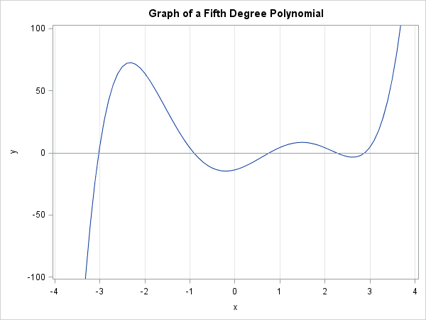
Let's see how this technique works in practice. The following SAS/IML function evaluates a fifth-degree polynomial by using Horner's method. The graph of the polynomial (shown to the left) reveals that it has roots near the values {-3, -1, 1, 2.5, 3}. The MeshEval function evaluates the polynomial at evenly spaced points and returns the subintervals on which the polynomial changes signs:
proc iml;
/* Evaluate fifth-degree polynomial function. Make sure this function can
   evaluate a vector of x values.
   To generalize, write:  start Func(x) global(p);   */
start Func(x);
   /* c5*x##5 + c4*x##4 + ... + c0 */
   p = {1 -2 -10 20 9 -14};       /* Coefficients: p[1]=c5, p[2]=c4, etc */
   y = j(nrow(x), ncol(x), p[1]); /* initialize to coef of largest deg */
   do j = 2 to ncol(p);           /* Horner's method of evaluation */
      y = y # x + p[j];
   end;
   return(y);
finish;

/* Evaluate function 'Func' and return intervals where function
   changes sign. Specify a large interval [a,b] and the number, n,
   of equally spaced subdivisions of [a,b].    */
start MeshEval(ab, n);
   x = ab[1] + range(ab)/n * (1:n);         /* n values of x */
   y = Func(x);
   difSgn = dif(sign(y));
   idx = loc(difSgn=2 | difSgn=-2);
   if IsEmpty(idx) then return ( {. .} );
   return( x[idx-1] || x[idx] );
finish;

ab = {-10 10};                /* search for roots on this big domain */
n = 100;                      /* break up into n smaller intervals */
intervals = MeshEval(ab,n);   /* intervals on which the function changes sign */
F = Func(intervals);
print intervals[c={"a" "b"} L=""] F[c={"F(a)" "F(b)"} L=""]; |
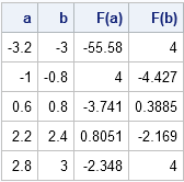
The table shows five bounding intervals on which the function changes signs. Because the function is continuous, there are roots in the intervals [-3.2, -3], [-1, -0.8], [0.6, 0.8], [2.2, 2.4], and [2.8, 3]. You can use the FROOT function to find the roots in each bounding interval:
roots = froot("Func", intervals);
print roots; |
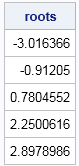
The FROOT function found all five roots, one root per bounding interval.
How to find the roots of 4,000 functions?
Returning now to the problem asked in the SAS Support Community, the infrastructure is in place to solve for the roots of an arbitrary number of polynomials. All you need to do is add a GLOBAL statement to the START statement and pass in p as a global variables that contains the coefficients. For each set of coefficients in the file, assign p and call the MeshEval and FROOT functions.
In fact, the Func function is written so that it can evaluate a polynomial of any degree, so the same function will work regardless of the number of elements in the p vector.
This approach will always succeed for odd polynomials because you can always find a bounding interval. However, it might not find all roots, and this approach can fail for an arbitrary function. For example, the quadratic polynomial fx) = x2-ε2 has roots at ±ε. When ε is small, the EvalMesh function might not find a bounding interval unless n is very large. If you are sure that the function has a real root, but EvalMesh does not find it, you can iteratively increase the value of n and call EvalMesh until the root is found.
The post Finding roots: Automating the search for an initial guess appeared first on The DO Loop.
Please comment on the article here: The DO Loop
